Attention is all you need

Induction vs Transduction

In supervised learning, where training samples are labeled with ground-truth, induction is the application of knowledge, or statistical inference, gained from the training set to a specific and finite set of unseen test samples. In contrast, transduction consists in exploiting the patterns in both the training and the testing set, even though the test samples are unlabeled.

The major difference between the two approaches is that induction results in a predictive model, one that is trained once on a finite data set and applied to novel test samples, while transduction requires seeing the entire collection of data points every time that new test samples are introduced.

In the context of sequence-to-sequence or language modeling, the problem is defined as transductive by nature. This is because every point in the sequence, or every token in a sentence, is needed to compute the output. The transformer is defined as transductive because each input relates to every other inputs and it is not done in a sequential manner that would allow induction, although it can abstractly be viewed as an inductive model because of the long-term memory induced by the MLP components of Transformer-encoder blocks.

Attention, attention!

The Scaled Dot-Product Attention function

A simple attention module

\[s_i = \sum_j w_j x_{ij}\] \[w_j = \frac{e^{z_j}}{\sum_k e^{z_k}}\]

Effectively, the attention mechanism can be seen as a multiplicative module that switches on or off the components of a variable. The weights vector, \(w\) , can be interpreted as probabilities which mask out or attenuate parts of the input. When this module is applied to a sequence of variables as such:

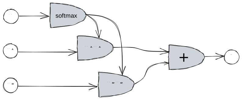where \(w\) is computed from \(z\) through the softmax function. Using the logistic function allows to smoothly blend variables by disabling or enabling specific components of each.

In short, attention within a neural network can be used to switch on or off parts of the network, or components of a variable, via multiplicative interaction.

The attention mechanism

The Attention mechanism, the central part of many transductive models, consists in modeling the relationships between points in any dimensional space without regards to their distance. This aspect is particularly attractive because it enables long-distance dependencies between points in a sequence or set.

An attention function can be described as mapping a query and a set of key-value pairs to an output, where the query, keys, values, and output are all vectors. The output is computed as a weighted sum of the values, where the weight assigned to each value is computed by a compatibility function of the query with the corresponding key.¹

There are mainly two versions of attention: additive attention and multiplicative (or dot-product) attention. The former computes the compatibility function via a 1-hidden-layer MLP, which is rather costly, while the latter is a dot-product that can be highly optimized. The Transformer architecture uses a scaled dot-product attention function.

The scaled dot-product

As stated above, the inputs are queries and key-value pairs, where the queries and keys are vectors of dimension \(d_k\) and the values are vectors of dimension \(d_v\).

The scaled dot-product attention is defined by Vaswani et al.¹ as:

\[\text{Attention}(Q,K,V) = \text{softmax}(\frac{QK^T}{\sqrt{d_k}})V\]

With \(Q\), \(K\), \(V\) being the query, key and value vectors packed into matrices for more efficient computation, such that the output weights form a matrix. Those weights represent how each value is relevant to each query-key pair.

A vector version of the attention function is defined as:

\[y_i^h = Att(q_i^h, K^h)V^h\] \[Att(q_i^h, K^h) = \text{softmax}{(\frac{q_i^h \dot K^h}{\sqrt{d_k}})}\]

So what are those queries, keys and values exactly?

The idea is that there is a difference between what attention should be paid to and where the information should be extracted. This is the reasoning behind the key-value pairing: we’re paying attention to the keys and we’re extracting information from the values. In the end, for the case of NLP, the queries, keys and values are all the same words of the input sequence (for the encoder part of the Transformer at least). But this attention function is flexible and you could very well decide to learn the queries or use different key-value pairs.

The dot-product

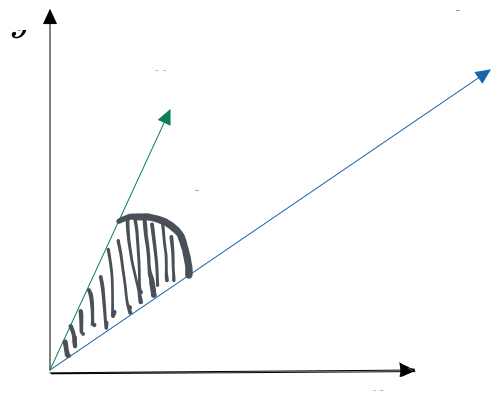
The dot-product between two vectors \(\mathbf{a}\) and \(\mathbf{b}\) is defined as:

\[\mathbf{a} \cdot \mathbf{b} = \lVert \mathbf{a} \rVert \lVert\mathbf{b}\rVert \cos \theta\]

where \(\theta\) is the angle between \(\mathbf{a}\) and \(\mathbf{b}\). This means that vectors that have a similar direction will have a high dot-product relative to their scale. It is important to scale it down so that the dot-products are normalised, and a factor of \(\frac{1}{\sqrt{d_k}}\) is used since larger values of \(d_k\) tend to push the Softmax function into regions where it has extremely small gradients: this is because the dot-product between the vectors \(q\) and \(k\) is: \(q \cdot k = \Sigma_{i=1}^{d_k} q_i k_i\), and so it scales linearly by \(d_k\). Therefore it is a countermeasure to the vanishing gradient problem.

The Softmax function

Softmax is defined as:

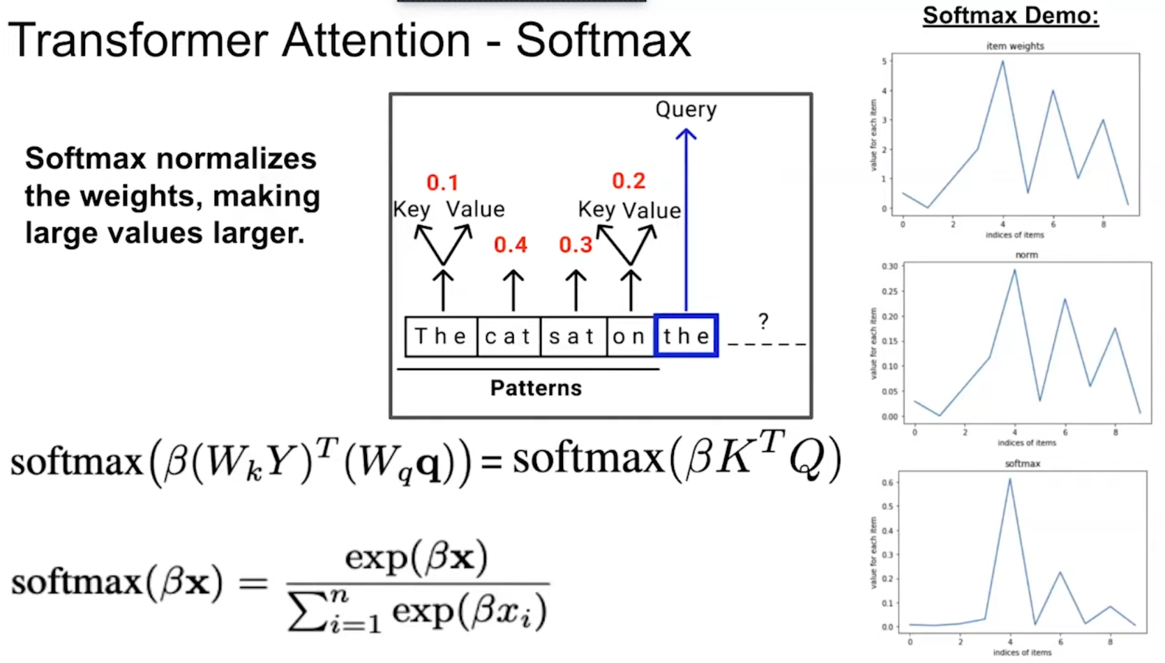
\[\sigma(\vec{z})_i = \frac{e^{z_i}}{\sum_{j=1}^{K}e^{z_j}}\]

where \(z_i\) are the elements of the input vector, and \(e\) is the Euler number of the exponential function. The denominator is the normalization term which ensures that all the output values of the function will sum up to \(1\), thus constituting a valid probability distribution. Softmax normalizes the weights, but it makes large values larger via the exponential function, as the following figure² illustrates:

Multi-head Attention

In practice, the Transformer architecture does not perform single attention on the entire queries, keys and values. Instead, it applies a linear projection to those vectors such that

\[Q, K, V = QW^Q, KW^K, VW^V.\]

However, this operation is done \(h\) times with each different weight matrices, so that it can learn different representations. This becomes useful when the scaled dot-product attention is computed in parallel for each resulting \(Q, K, V\) matrices, before concatenating the final attention weights.

¹

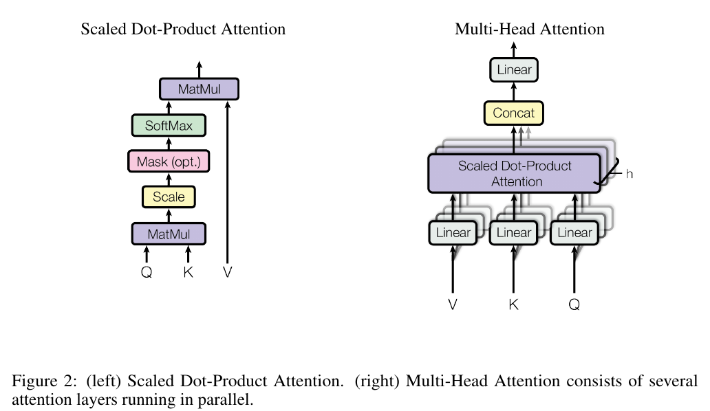
As defined by Vaswani et al.¹,

\[\text{MultiHead}(Q,K,V) = \text{Concat(head}_1, \ldots, \text{head}_h)W^O\] \[\text{head}_i = \text{Attention}(QW_i^Q, KW_i^K, VW_i^V)\]

Multi-head attention allows the model to jointly attend to information from different representation subspaces at different positions. With a single attention head, averaging inhibits this.¹

We can use the analogy of the layered structure of CNNs to motivate Multi-Head attention: as we go deeper in the network, the receptive field increases.

The Transformer architecture

Now that we understand attention, and more specifically the Multi-Head Attention mechanism, we can insert it into its context in the following Transformer encoder-decoder architecture: 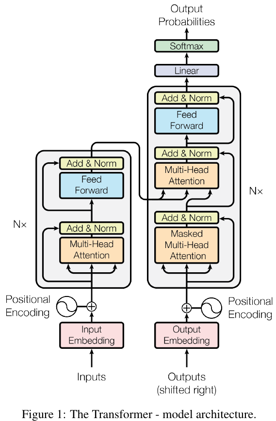¹

However there are a few things that we missed:

• Positional Encoding: it is helpful for the transformer to have a notion of position and order for the tokens in the sequence of inputs, therefore an optionally learned position embedding is added to the input/output embeddings. The original Transformer architecture uses fixed sine and cosine functions of different frequencies, but the Vision Transformer², for instance, uses learned embeddings that are appended to the latent embeddings.
• Feed Forward Layer: those fully-connected ReLU feed-forward networks are applied to each position separately, as a two-layer MLP with different parameters for each layer of the Transformer. They implement a long term memory version of attention. In normal attention, the keys and values are a function of the receptive field (current inputs). This long term attention however is independent of the particular inputs, it will store longer term memories across the whole training.³
• Layer Norm: Important for the cosine similarity, but can be improved with L2 norm.³

Auto-associativity vs hetero-associativity

What’s the difference between autoregressive transformers and hetero-regressive transformers? Basically, in an autoregressive or auto-associative transformer the keys point to other keys or even themselves (therefore the queries are the keys as well), and in a hetero-associative setting where you want to associate A to B or predict the next token in a sequence, the keys point to values in a different set.³

1. Attention Is All You Need (Vaswani et al.) ↩︎ ↩︎² ↩︎³ ↩︎⁴ ↩︎⁵ ↩︎⁶

2. An Image is Worth 16x16 Words: Transformers for Image Recognition at Scale (Dosovitskiy et al.) ↩︎ ↩︎²

3. Attention Approximates Sparse Distributed Memory ↩︎ ↩︎² ↩︎³