A Gentle Introduction to Meta-Learning
A Gentle Introduction to Meta-Learning — notes by Théo Morales
Check out my PyTorch implementation of MAML!
Deep Neural Networks are used to address complex recognition or classification problems, but they need enormous datasets to train the considerable number of trainable parameters within the network. As a result, the training process is prolonged. However, reducing the training dataset size is not an option, as a large network may recognise only items in the training set and not the underlying class of items. This problem is called overfitting, and while there are some techniques to address this, they result in even slower training and need to be tuned manually.
In the classical approach, a Deep Neural Network is trained using a fixed data set, after which the trainable parameters of the network are frozen, which prevents further learning. If we allowed the network to learn from new data, this learning would eventually overwrite the trainable parameters, and the network would only recognise the classes described by the new data.
In contrast to Deep Neural Networks, humans learn new concepts efficiently with few samples by associating past knowledge with similar patterns. Ideally, a learning algorithm should attain human levels of performance. To achieve this speed of learning, we need a different way to train Deep Neural Networks.
The first approach to this problem was “Transfer Learning”, which involves first learning from a very large data set training the last few layers on a different, but closely related task. The limitations of this approach are that the new items have to be very similar to the original items, and the problem of overfitting remains.
Other approaches aim to solve the “forgetting” problem by adding memory to Deep Neural Networks, or to solve the “manual tuning” problem by separately learning the update rule for the network parameters. These methods belong to a field of study called “Meta-Learning” which trains a Deep Neural Network to classify items based on the outputs of other Deep Learning Networks.
In meta-learning, the goal of the trained model is to quickly learn a new task from a small amount of new data.1
The idea of a task is central to Meta-Learning, and is defined as a small set of data points that come from the same distribution, such that multiple tasks share similarities but also have a structure independent of each other. For example, classifying images of different dog breeds can be seen as a multi-task problem, where each breed is a task with specific appearance features. All dog breeds share similar traits, such as having four legs, a tail, and a similar shape. Therefore all tasks are related.
Task definition in Meta-Learning
A generic notion of a learning task is defined1 as \(\mathcal{T}=\{\mathcal{L}(\mathbf{x}_1, \mathbf{a}_1, \ldots, \mathbf{x}_H, \mathbf{a}_H), q(\mathbf{x}_{1}), q(\mathbf{x}_{+1}\vert\mathbf{x}_t,\mathbf{a}_t),H\}\) with a loss function \(\mathcal{L}\), a distribution over initial observations \(q(\mathbf{x}_1)\), a transition distribution \(q(\mathbf{x}_{t+1}\vert\mathbf{x}_t, \mathbf{a}_t)\) and an episode length \(H\) (equal to 1 in i.i.d supervised problems). The model \(f(\mathbf{x})=\mathbf{a}\) may generate samples of length \(H\) by choosing an output \(\mathbf{a}_t\) at each time \(t\).
In the multi-task meta-learning scenario, the model should adapt to a distribution over tasks \(p(\mathcal{T})\), and it is trained (this is the phase called meta-training) to learn a new task \(\mathcal{T_i}\) drawned from \(p(\mathcal{T})\) from only \(K\) samples drawn from \(q_i\) and feedback \(\mathcal{L}_{\mathcal{T_i}}\) generated by \(\mathcal{T_i}\). It is then tested on new samples from \(\mathcal{T_i}\); this is called meta-testing. Thus, the test error on sampled tasks \(\mathcal{T_i}\) for the model \(f\) serves as the training error of the meta-learning process.
Thus, for Meta-Learning to be applicable, all tasks must share similarities and the training and testing conditions must be consistent. If a Deep Neural Network were trained with an inconsistent number of examples for each task, the network would not learn to learn efficiently and it would have inconsistent performance across the different tasks.
One approach, called Model-Agnostic Meta-Learning (MAML), trains a Deep Neural Network simultaneously on a group of tasks. This way, MAML trains the network to learn common patterns across similar tasks. The network encodes general knowledge that enables it to learn a novel concept rapidly and with few examples. MAML has an outer loop and an inner loop.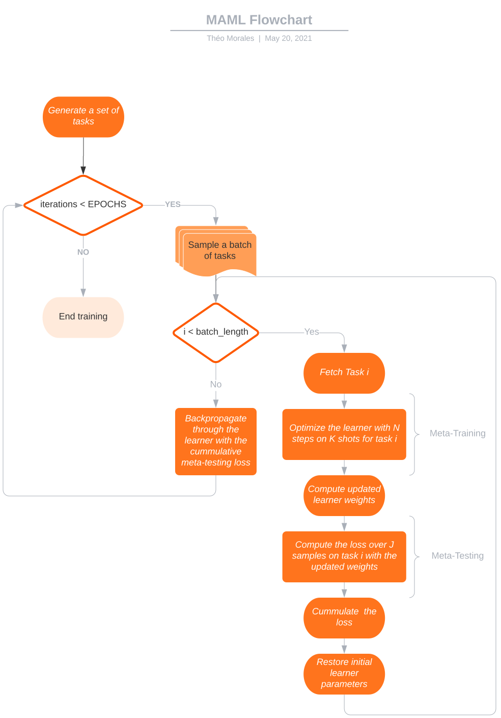 The inner loop trains the network in a classical manner, as a single-task objective, on a small set of examples then evaluates this network on a slightly larger set of validation examples. Between each single-task training, the network’s parameters are reset to their initial inner loop state at a step t, as to evaluate the training efficiency on each task from the same initial parameter values. The loss, a value representing the prediction error on the validation examples, is accumulated over a batch of tasks in this inner loop training phase. A large loss would indicate a poor choice of initial parameter values, resulting in inefficient training for any given task. Therefore, this loss represents the goodness of network initialization (the value of its parameters before training for a new task) for fast training with few examples on a novel task. In the outer loop, this total loss is directly used to derive the updated model parameters, with an algorithm such as stochastic gradient descent which computes the right change in each parameter’s value that decreases the error value. In essence, it can be seen as finding the right spot in a valley - the network initialisation - such that the distance to each mountain’s peak - the inner loop training loss - would be minimal: finding that spot is done in the outer loop, with the total distance to each peak calculated in the inner loop. At every training step, a new valley with a different set of mountain peaks is given (a batch of tasks), and the starting spot (the network parameters) gets better by each iteration.
An in-depth view of the MAML algorithm
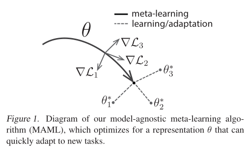 The intuition behind the proposed approach, of learning the parameters of any standard model via meta-learning, is that some internal representations are more transferrable than others.
The overall goal of the algorithm is to find model (optimizee) parameters that are sensitive to changes in the novel task loss (small changes induce large improvements), on any task drawn from \(p(\mathcal{T})\). This should have the effect of capturing internal features that are broadly applicable to all tasks in \(p(\mathcal{T})\).
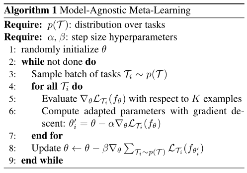 As seen on Algorithm 1, the step size \(\alpha\) may be fixed or meta-learned. The meta-objective is as follows:
The meta-gradient is computed here, as being the gradient of the gradient of each task.
The clever trick here is that meta-optimization is performed over the model parameters \(\theta\) whereas the objective is computed using the updated model parameters \(\theta^\prime\), suich that it optimizes the model parameters in a way that one or a small number of gradient steps on a new task will produce maximally effective behavior on that task.
Line 8 of Algorithm 1 shows the stochastic gradient descent update for the model parameters \(\theta\) across tasks. This is the meta-gradient! Basically on line 8, the gradient of the sum of the loss of each task is computed with respect to \(\theta\). The losses are computed with the updated model \(f(\theta^\prime)\), which means that \(\nabla_\theta\) on line 8 represents the amount of change on the loss when the model is updated! Therefore the updated meta-gradient should induce the largest possible change on the loss function of each task, and that is why this paper is so clever. It is like looking in the future, going back to the present, and setting the exact step size that will land the model on the minima. This also ensures that the new meta-gradient will not greatly improve the loss on one task to the detriment of another task.
To compute the meta-gradient, an additional backward pass through \(f\) is necessary to compute the Hessian-vector products (one first pass for \(\nabla_\theta \mathcal{L}_\mathcal{T_i}(f_\theta)\) and another pass for that gradient with respect to \(\theta\)). In their experiments, they compare this to just using a first-order approximation. Note that a first-oder approximation means a Taylor series of expansion to the first order only, not a first derivative!
Unlike previous work (such as Andrychowics et al., 2016), the algorithm does not expand the number of learned parameters nor constrains the model architecture (an RNN or a Siamese network), and it can be readily combined with MLPs, CNNs or RNNs. It can even be used with non-differentiable RL objectives. That is mainly why MAML was a breakthrough in meta-learning!
Experimental results show that MAML is better at multi-task learning for classification, regression and even reinforcement learning problems. The main advantage of MAML over Transfer Learning is that it is much more efficient on task adaptation, the training efficiency for a given unseen task, with respect to training iterations and data regime (the amount of training data available). MAML is model agnostic, meaning that it is a generic method for training a wide range of different types of Deep Neural Networks. In fact, it can bring significant value in contexts where gathering training data is costly and where the problem to solve changes often. For instance, a security system could be pre-trained with meta-learning so that it would be able to classify new persons or pets as “non intruders”, given only a few shots. Nevertheless, meta-training remains time-consuming and demanding, although MAML is able to flexibly compromise accuracy for training speed on novel tasks. Recent work has shown promising results in this direction, and meta-learning methods are beginning to reach accuracy levels close to traditional single task training methods.