The Jacobian matrix

The Jacobian essentially represents what a multivariable function looks like locally (when zooming in on a specific point), as a linear transformation.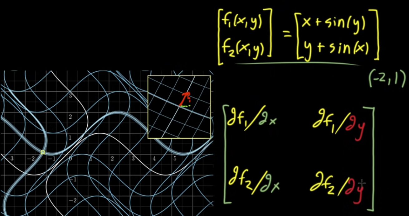

When taking a point \(\mathbf{v}\) to be transformed by the (non-)linear transformation \(F\) as \(\mathbf{u} = F \mathbf{v}\) where

\[F = \begin{bmatrix} f_1(x,y) \\ f_2(x,y) \end{bmatrix} \text{,}\]

the change in the output space in \(x\) is the change of \(f_1\) w.r.t \(x\) plus the change of \(f_1\) w.r.t. \(y\), and the change in \(y\) (still in the output space) is the change of \(f_2\) w.r.t. \(x\) plus the change of \(f_2\) w.r.t. \(y\).

As such, the matrix describing these changes in \(x\) and \(y\) is the Jacobian matrix, expressed as:

\[\begin{bmatrix} \frac{\partial f_1}{\partial x} & \frac{\partial f_1}{\partial y} \\ \frac{\partial f_2}{\partial x} & \frac{\partial f_2}{\partial y} \end{bmatrix}.\]

This matrix defines the new basis vectors for a linear transformation. It is linear because partial derivatives describe infinitesimally small changes in the input, which is like zooming in on the a point in the non-linear transformation.

Takeaway When evaluated at a point, the Jacobian matrix shows what the linear transformation looks like locally.

In linear algebra, the Jacobian is the matrix of first-order partial derivatives for vector-valued functions.